
Abstract
BACKGROUND AND PURPOSE: The new 3.0-T imagers theoretically yield double the signal-to-noise ratio (SNR) and spectral resolution of 1.5-T instruments. To assess the possible improvements for multivoxel 3D proton MR spectroscopy (1H-MRS) in the human brain, we compared the SNR and spectral resolution performance with both field strengths.
METHODS: Three-dimensional 1H-MRS was performed in four 21–29-year-old subjects at 1.5 and 3.0 T. In each, a volume of interest of 9 × 9 × 3 cm was obtained within a field of view of 16 × 16 × 3 cm that was partitioned into four (0.75-cm-thick) 16 × 16-voxel sections, yielding 324 (0.75-cm3) signal voxels per examination.
RESULTS: In an acquisition protocol of approximately 27 min, average voxel SNRs increased 23–46% at 3.0 versus 1.5 T in the same brain regions of the same subjects. SNRs for N-acetylaspartate, creatine, and choline, respectively, were as follows: 15.3 ± 4, 8.2 ± 2.2, and 8.0 ± 2.0 at 1.5 T and 22.4 ± 7.0, 10.1 ± 3.5, and 10.1 ± 3.6 at 3.0 T. Spectral resolution (metabolite linewidths) were 3.5 ± 0.5 Hz at 1.5 T versus 6.1 ± 1.5 Hz at 3.0 T in approximately 900 voxels. Spectral baselines were noticeably flatter at 3.0 T.
CONCLUSION: Expected gains in SNR and spectral resolution were not fully realized in a realistic experiment because of intrinsic and controllable factors. However, the 23–46% improvements obtained enable more reliable peak-area estimation and an 1H-MRS acquisition approximately 50% shorter at 3.0 versus 1.5 T.
All major commercial manufacturers offer MR imagers with magnetic fields (B0) stronger than 1.5 T. Although more powerful 4-, 6-, 7-, and even 8-T full-body instruments are currently used, the most common higher-field-strength systems operate at 3.0 T. The rationale for the higher B0, so far, has almost exclusively been for functional MR imaging (1). The inevitable proliferation of higher-field-strength systems raises the question of whether an increased B0, with its associated cost and technical complications, will benefit other MR applications, such as in vivo proton MR spectroscopy (1H-MRS).
For MRS, although linear increases in the signal-to-noise ratio (SNR) per unit time and spectral resolution are predicted with increasing B0 (2–5), neither actually may be realized. Obstacles that can be addressed, such as lower-sensitivity coils and poorer shimming, may combine with intrinsic limitations, such as shorter T2s and longer T1s of metabolites, to nullify either or even both advantages (2, 6). Furthermore, larger chemical-shift misregistration errors at the higher B0s could degrade their usefulness for MRS to below that of the mature, optimized clinical 1.5-T imagers.
The possible advantages versus limitations of 3-T imagers motivated us to compare whether a benefit to MRS can be realized and if so, to determine its extent. To that end, we performed the same 3D 1H-MRS examination in similar regions in the brains of the same four age-grouped volunteers at 1.5 and 3.0 T. The goals were quantitative evaluation of the SNRs and local linewidths of N-acetylaspartate (NAA), creatine (Cr), and choline (Cho) and qualitative evaluation of the perceived quality of their spectra.
Methods
Human Subjects
Four healthy volunteers, three women and one man aged 20–29 y, participated in this comparison. Since the experiments were performed with two different imagers, as long as 2 wk elapsed between examinations at each field strength per volunteer. We assumed that no MR-detectable changes occurred in their brains over such a short period. All volunteers were briefed on the procedures and provided written consent on forms approved by the institutional review board.
Common-Field-Strength 1.5-T Imager
Lower-field experiments were performed with a 1.5-T system in its standard configuration for human subjects. The Q factor of its circularly polarized head coil was 60/300 (loaded/unloaded) with a preamplifier that had a 1.2-dB noise figure. A 3D chemical shift imaging (CSI)–based auto-shim yielded <10 Hz full-width at half-maximum (fwhm) whole-head water lines (7). Since B0 inhomogeneities dominated this line, it narrowed to 6 Hz in the volume of interest (VOI), enough for one chemical shift selective (CHESS) pulse and a band-selective inversion with gradient-dephasing (BASING) pulse (Fig 1) to suppress the water signal 1000-fold (8, 9).

Schematic of the hybrid HSI-CSI localization sequence. A 25.6- or 15-ms, 60- or 120-Hz water suppression at 1.5 or 3.0 T was followed by VOI excitation. The PRESS 5.12-ms 90° pulse also performed fourth-order HSI (HSI) along ZIS with 3 or 4.5 mT/m gradients at 1.5 or 3.0 T, respectively, followed 26.07 and 98.69 ms later by 10.24 ms SLR 180° pulses with 1 mT/m. Localization along XLR and YAP was 16 × 16 2D CSI. A 25.6- or 15-ms gaussian 180° BASING pulse was applied between the two SLR pulses for extra water suppression
High-Field-Strength 3-T Imager
These experiments were performed with a Medspec 30/80 unit (Bruker Medical, Ettlingen, Germany). It comprised all-commercial components to comply with approval for investigational use in human subjects. The Q factor of its circularly polarized birdcage head coil was ≈250/1000 (loaded/unloaded), and the noise figure of its preamplifier was 1.7 dB. The Bruker implementation of the Gruetter FASTMAP auto-shim method yielded <7 Hz fwhm water lines from the VOI (10). Three CHESS pulses and a BASING pulse suppressed the water signal of the VOI approximately 1000-fold.
3D 1H-MRS Sequences
The same 3D 1H-MRS sequence (Fig 1) was used at both field strengths (11, 12). A 9 × 9 × 3-cm left-right (LR) × anteroposterior (AP) × inferosuperior (IS) VOI was excited by using point-resolved spectroscopy (PRESS) with a TE of 135 ms (13). The 16LR × 16AP × 3IS-cm field of view (FOV) was partitioned into four IS sections by using Hadamard spectroscopic imaging (HSI) and 16LR × 16AP axial voxels arrays by using 2D CSI. Section-selection gradients for the HSI 90° and the Shinnar–Le Roux (SLR) 180° pulses were 3 and 1 mT/m, respectively, at 1.5 and 4.5 T and were both 1 mT/m at 3.0 T. Overall, 324 voxels (9LR × 9AP × 4IS), each 0.75 cm3, were formed in the VOI. A TR of 1.6 s, optimal for the 1.3–1.4-s T1s of brain metabolites at 1.5 and 3.0 T, was used throughout (14–16). Consequently, MRS required 27 min at either field strength.
Image-Guided MRS and Postprocessing
The position and size of the VOI and the localization grid were interactively image guided in three perpendicular planes to output the shaped radio-frequency waveforms seen in Fig 1 (11, 17). The MR imaging and 1H-MRS data were processed off-line by using in-house software. Residual water was removed in the time domain (18), a matched Lorentzian filter (3 Hz at 1.5 T, 6 Hz at 3.0 T) was applied, and 2D voxel-shift was used to align the CSI grid with the VOI. Fourier transforms were performed in the temporal and two spatial dimensions, and Hadamard transform was performed in the third. No spatial filters were applied. Finally, the spectra were automatically corrected for frequency and zero-order (and first-order) phase shifts by using NAA (and Cho) peaks in voxels where either (or both) were available.
Results
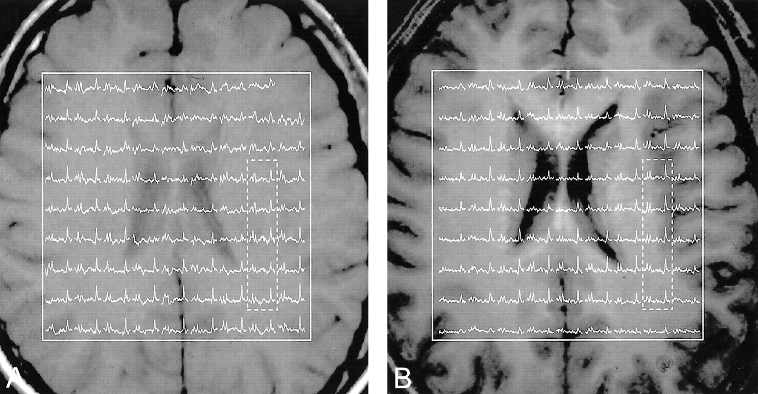
The position of the VOI was image guided within 2–3-mm registration uncertainty to the same anatomic landmarks in each volunteer at 1.5 and 3.0 T (Fig 2). The 9 × 9 spectra matrices in the VOIs in Figure 2 correlated well with the underlying anatomy of the corresponding images, as manifested in reduced signals where the voxels involved ventricles (19). The real part of the five 1H spectra highlighted in Figure 2 are expanded for greater detail and shown for comparison in Figure 3, which is scaled for the same maximum NAA peak height.

Corresponding (within 2–3 mm IS) axial T1-weighted MR images from the section richest in anatomic features from the same subject. Both are superimposed with the outline of the 9 × 9-cm VOIs and the real part of the corresponding 9 × 9 1H-spectra matrices. The horizontal (1.8–3.5-ppm) scale is common to both fields.
A, Examination at 1.5 T.
B, Examination at 3.0 T.

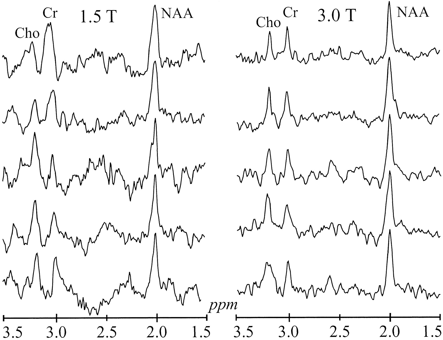
Five spectra from the corresponding dashed boxes in figure 2 scaled to the same maximum NAA peak height. Note an improved Cr-Cho spectral resolution, better SNR, and flatter baseline between 2 and 3 ppm at 3.0 versus 1.5 T
In all, 364 voxels per VOI among the four subjects, or a total of 1296 voxels, were obtained with each field. Average metabolite SNRs were calculated as follows: 1) The amplitudes, Sij, (i = NAA, Cho, or Cr) were obtained in each voxel, with j = −1296. 2) The standard deviation of the noise, σnoise, was estimated from the signal-free −1 to −2 ppm region. 3) Voxels in which Sij was less than 6σnoise or where severe baseline distortions from residual water or fat were incurred were rejected, leaving approximately 900 of the 1296 voxels for analysis. 4) The voxel SNR, Sij/σnoise (20), was computed for each metabolite, and the SNRs were averaged. The averages and SD of each metabolite at either B0 are shown in the Table.
Average voxel linewidths and SNRs from approximately 900 voxels
The apparent linewidths of the metabolites at each field strength in each signal voxel and volunteer were calculated with the parametric spectral modeling and least-squares optimization method of Soher et al (21). This process makes use of a priori spectral information and includes automatic phasing, nonparametric characterization of baseline signal components, and a Lorentz-Gauss line-shape assumption. Average fwhm at each field strength for the 900 or so signal voxels in the four volunteers were 3.5 ± 0.5 Hz at 1.5 T and 6.1 ± 1.5 Hz at 3.0 T (Table).
Discussion
SNR Performance
In a realistic MRS experiment, with TE > 0 and TR < ∞, the doubling in SNR with use of a 3.0 versus 1.5 T (3, 4) could not be achieved because of the longer T1s and shorter T2s of the metabolites. Luckily, T1s reported for NAA, Cho, and Cr at 3.0 T were similar to those published for 1.5 T (1.3–1.4 s) (14, 16, 22). Unfortunately, T2 values, which are 350–500 ms for NAA at 1.5 T, depending on tissue type (white matter or gray matter), were reduced to 200–300 ms at 3.0 T (14, 16, 22). Given the similar T1s and different T2s at 1.5 and 3.0 T, for equal TRs and TE > 0, the ratio between the signals is calculated as follows:  Therefore, the observed 23–46% gains shown in the Table and Figure 2 are within those of the theoretical prediction. Note that the σ/average SNRs of the metabolites, 25–30% at each B0 in the Table, most likely reflect the heterogeneity of the brain rather than intrinsic variability of the method.
Such gain is notable given the variations reported between normal and diseased brains, as follows: approximately 50% in cancer, less than 20% for human immunodeficiency virus infection and focal epilepsy, and approximately 30–70% in multiple sclerosis and Alzheimer disease (23). It will enable us to discern changes earlier in response to disease progression or treatment. Alternatively, SNR can be traded for shorter sessions: For example, to retain the lowest SNR of 1.5 T (Cho) at 3.0 T, the acquisition could be shortened 26%, from 27 to 17 min, a substantial time savings.
Spectral Resolution
Magnetic field inhomogeneities (ΔB0) arising from susceptibility differences (Δχ) at tissue-air and tissue-bone interfaces broaden resonance lines (24, 25). These macroscopic regional effects are especially pronounced in the frontal and temporal lobes above the sinuses, in the vicinity of the auditory canals, and near the skull (24–26). They can be as large as 2.0 ppm in a 2 × 2 × 2-cm voxel (25), they cannot be completely removed with the first- and second-order shims found in clinical MR imagers (10), and they linearly worsen with increasing B0.
The fact that the linewidth is “only” twice as wide as that of its individual voxels—that is, approximately 3.5 and 6.1 Hz at 1.5 T and 3.0 T (Table, Fig 3)—indicates that the local ΔB0 directions (fortunately) are random, as Hansen et al (27) pointed out. One of the sources and locale of this broadening is evident in Figure 2, where the first (anterior) row of spectra, situated above the sinuses, displays broader NAA linewidths compared with the last (posterior) row, which is the furthest from known severe Δχ sources.
Despite shorter T2s and roughly twofold local and global susceptibility broadening, the chemical shift doubling at 3.0 T yields better voxel spectral resolution at the higher field strength. This finding is reflected by baseline Cr–Cho separation at 3.0 T in the voxels of Figures 2 and 3. The 0.2-ppm chemical shift between Cr and Cho is constant at either field strength. However, since the spectra are acquired and processed in hertz, not parts per million, the doubled chemical shift at the higher field strength increases the absolute hertz separation between these lines. The overall result is improved spectral resolution at 3.0 T, despite a very similar linewidth and/or separation ratio at each field strength (Table, Fig 3). In addition, the slightly less than doubled linewidth in the local voxels (≈6.1 Hz at 3.0 T vs ≈3.5 Hz at 1.5 T) contributed further to the improvement in spectral resolution at the higher field strength. This finding can be attributed to slightly better local shimming achieved at 3.0 T in this study.
The 3.0 T spectra also are distinguished by a flatter baseline between the NAA and Cr peaks (2–3-ppm region in Fig 2). Because of an intermediate TE (135 ms) and the decrease in T2s of the general metabolites with increasing field strength, the broad resonances were almost completely dephased at 3.0 T. The resulting flatter baseline aids in more reliable estimation of peak area, as Kreis et al (14) pointed out.
Spatial Resolution
With 3- and 4.5-mT/m gradients used in the HSI direction, the ≈2-ppm 1H chemical shift between lactate and Cho yields a relative position shift of as much as 0.10 and 0.13 cm (13% and 18% of the 0.75-cm-thick sections) at 1.5 and 3.0 T, respectively. CSI localization in the planes of the sections caused no chemical shift errors. No fat contamination was present upfield from NAA at either B0, qualifying both for studies of abnormal alanine or lactate in tumors, acute plaques of multiple sclerosis, radiation damage, or stroke (23).
Conclusion
Although high-field-strength instruments are relatively new compared with the optimized, mature 1.5-T instruments, their performance benefits for MRS already are evident. Specifically, when sequence, shim, and anatomy are approximately equal, improvements of about 20–50% can be realized in SNR per unit time and spectral resolution. These advantages allow shorter examinations and better quantification, especially for the adjacent Cr and Cho peaks.
Footnotes
1 Supported by European Union Grant BIOMED 2 CT96-0861 (E.M.) and Grants NS33385 and NS37739 from the National Institutes of Health (O.G.).
2 Address reprint requests to Oded Gonen, Department of Radiology, New York University School of Medicine, 550 First Avenue, New York, NY 10016.
References
- Received February 1, 2001.
- Copyright © American Society of Neuroradiology


