
Abstract
BACKGROUND AND PURPOSE: Exploring the directionality of neural information in the brain is important for understanding brain mechanisms and neurodisease development. Granger causality analysis and the metabolic connectivity map can be used to investigate directional transmission of information between brain regions, but their differences in depicting functional effective connectivity are not clear.
MATERIALS AND METHODS: Using the Monash rs-PET/MR imaging data set, we conducted Granger causality and metabolic connectivity map analyses of the dopamine reward circuit in the brain. The dopamine reward circuit is a well-known system consisting primarily of the bilateral orbital frontal cortex, caudate, nucleus accumbens, thalamus, and substantia nigra. We validated these circuit pathways using Granger causality and the metabolic connectivity map for identifying effective connectivities against a priori knowledge by testing the significance of directed pathways (P < .05, false discovery rate–corrected).
RESULTS: We found 3 types of effective connectivities in the dopamine reward circuit: long-range, neighborhood, and symmetric. Granger causality analysis revealed long-range connections in the orbital frontal cortex–caudate and orbital frontal cortex–nucleus accumbens regions. Metabolic connectivity map analysis revealed neighborhood connections in the nucleus accumbens–caudate, substantia nigra–thalamus, and thalamus-caudate regions. Metabolic connectivity map analysis also found symmetric connections in each of the bilateral nucleus accumbens, caudate, thalamus, and orbital frontal cortex–caudate regions. Different patterns in directional networks of the dopamine reward circuit were revealed by Granger causality and metabolic connectivity map analyses.
CONCLUSIONS: Granger causality analysis primarily identified bidirectional cortico-nucleus connections, while the metabolic connectivity map primarily identified direct connections among neighborhood and symmetric regions. The results of this study indicated that investigations of effective connectivities should use an appropriate analysis method depending on the purpose of the study.
ABBREVIATIONS:
- BOLD
- blood oxygen level–dependent
- BG
- basal ganglia
- CAU
- caudate
- DA
- dopamine
- EC
- effective connectivity
- FC
- functional connectivity
- FDR
- false discovery rate
- GC
- Granger causality
- GCI
- Granger causality index
- MCM
- metabolic connectivity map
- NAc
- nucleus accumbens
- OFC
- orbital frontal cortex
- SN
- substantia nigra
- THA
- thalamus
The human brain has been recognized as a continuously communicating dynamic network.1 Intrinsic activities in structures as small as neurons can be analyzed with functional connectivity (FC) to identify functional brain networks. However, the directionality of the interactions within the brain networks built from these correlations cannot be determined. Effective connectivity (EC) provides the directional or causal relationships among brain region transmissions and can be used to explore these communications.2 Understanding the directionality of brain networks provides insight into the diagnosis and treatment of neurologic or mental diseases, such as Alzheimer disease,3 schizophrenia,4 and addiction.5
Granger causality (GC) analysis is a statistical method that adopts a linear vector autoregressive model of stochastic time-series data. GC was proposed for use in economics, but its use in fMRI studies of brain disorders has revealed the directionality of transmissions among brain regions.5⇓⇓-8
In studying the metabolic directionality among brain regions, Riedl et al9 proposed an approach called the metabolic connectivity map (MCM). The MCM is based on collecting energy consumption data in neuronal communications while simultaneously collecting PET and fMRI data. Most energy metabolism is dedicated to signaling and is consumed postsynaptically, in other words, at the target neurons.9⇓⇓⇓-13 Riedl et al scaled this to the system level with the assumption that an increase in local metabolism reflects an increase in afferent EC from source regions. They further hypothesized that the spatial correlations between metabolic activity and FC represent this EC spatial profile. In other words, the MCM reflects the correlation between the pattern of improved glutamate consumption and the pattern of improved blood oxygen level–dependent (BOLD) signals in the target region. The MCM has been used to identify altered EC within the default mode network for Alzheimer disease,3 reveal the stable bidirectional connection among early/higher visual regions of healthy cohorts,9 and study the cognition task-induced reconfiguration of whole-brain networks.14
BOLD signals measure indirect neuronal activities and are influenced by intermediate physiologic responses, including the cerebral metabolism rate of glucose/oxygen and the CBF/CBV. [18F] FDG-PET signals measure glucose metabolism in the brain, which is also influenced by the CBF/CBV. When PET and fMRI data are collected simultaneously, both the levels of glucose metabolism and BOLD signals are influenced by the simultaneous CBF and share a common basis in central neurophysiology. Human brain metabolic connectivity derived from [18F] FDG-PET is comparable with that derived from resting-state fMRI analyses.15,16 While these studies confirmed the comparability of nondirectional metabolism connectivity and BOLD connectivity, little was revealed about the relationship between glucose metabolic EC and fMRI EC. This issue has not been studied due to the lack of simultaneously acquired and aligned fMRI and PET data.
The novel advantages of integrated PET/MR imaging provide a new insight into understanding the dopamine (DA) reward circuit. The DA reward circuit consists of 3 pathways: the nigrostriatal pathway, along which the substantia nigra (SN) sends a dopaminergic projection to the dorsal striatum; the mesolimbic pathway, where the ventral tegmental area (VTA) sends a similar type of dopaminergic projection to the nucleus accumbens (NAc); and the mesocortical pathway, where dopaminergic projections are sent from the SN/VTA through the thalamus (THA) and the prefrontal cortex.17,18 There are rich bidirectional projection pathways among these brain regions19⇓-21 involved in the DA reward circuit. We chose brain areas involved in the DA reward system to validate the sensitivity and consistency of MCM and GC analyses and to identify the directed pathways among brain regions by ROI analysis.
Materials and Methods
Data Sets
The data for this study were obtained from the Monash rsPET-MR data set22⇓⇓-25 in the OpenNeuro database (https://doi.org/10.18112/openneuro.ds002898.v1.1.1). It is a simultaneous fMRI-functional PET data set acquired from young, healthy individuals at rest. Participants (n = 27, 21 women) were all right-handed, 18–23 years in age (mean age, 19 years), with 13–18 years of education (mean, 14 years) and no history of diabetes, diagnosed Axis-I mental illness, or cardiovascular illness.22 Participants underwent a 95-minute simultaneous MR imaging–PET scan in a 3T Biograph molecular MR imaging scanner (syngo VB20P; Siemens) as described previously.22,24 Briefly, [18F] FDG (average dose, 233 MBq) was infused over the course of the scan.22 During the first 30 minutes of the FDG infusion, T1 3D MPRAGE was acquired (Acquisition Time [TA] = 7 minutes 0.6 seconds, TR = 1640 ms, TE = 2.34 ms, flip angle = 8°, FOV = 256 × 256 mm2, voxel size = 1 × 1 × 1 mm3, 176 slices, sagittal acquisition). For the remainder of the scan, 6 consecutive 10-minute blocks of T2*-weighted echo-planar images were acquired (TR = 2.45 seconds, TE = 30 ms, FOV = 190 mm2, 3 × 3 × 3 mm3 voxels, 44 slices, ascending axial acquisition).
Image Preprocessing
The first 10-minute block of BOLD data, the corresponding 10-minute FDG-PET data, and the T1 3D MPRAGE data were used for structural segmentation and registration. Volumes from the PET data were reconstructed every 16 seconds, and the corresponding 10-minute data volume indexes were 129–165 for each participant. PET volumes were extracted and averaged to acquire static FDG-PET images.
The CONN toolbox (Version 20.b; https://web.conn-toolbox.org/)26 was used for BOLD data preprocessing. It is a functional connectivity toolbox based on the Statistical Parameter Mapping 12 toolbox (SPM; http://www.fil.ion.ucl.ac.uk/spm). The default preprocessing pipeline for volume-based analyses (“direct normalization to Montreal Neurological Institute space” pipeline in CONN) was used, including the following steps: 1) realignment and unwarping; 2) section-timing correction for interslice differences in acquisition time; 3) Artifact Detection Tools–based outlier detection (https://www.nitrc.org/projects/artifact_detect) to identify outlier scans for scrubbing; 4) segmentation of functional and anatomic images to gray and white matter and CSF tissue classes using SPM-unified segmentation and normalization procedures; and 5) normalization to 2-mm (functional) or 1-mm (anatomic) isotropic voxel size in Montreal Neurological Institute space. The functional images were smoothed using spatial convolution with a Gaussian kernel of 4 mm at full width at half maximum values. After preprocessing, functional data were further denoised, removing potential confounding effects in the BOLD signal, such as noise components from WM and CSF areas,27 estimated subject-motion parameters, scrubbing, and session effects.28 Temporal frequencies <0.008 Hz or >0.09 Hz were removed from the BOLD signal to focus on slow-frequency fluctuations while minimizing the influence of physiologic, head-motion, and other noise sources.29
ROI Definition and FC Analysis
FSL30 (http://www.fmrib.ox.ac.uk/fsl) built-in atlases were used to generate 10 ROIs in the DA reward system.31,32 Eight bilateral ROIs were extracted from the Harvard-Oxford probability atlas with a threshold set to 50% probability, then binarized into masks. The 8 bilateral ROIs were the thalamus (THA, left: 1139, right: 1129 voxels), (NAc, left: 70, right: 56 voxels), caudate (CAU, left: 444, right: 457 voxels), and orbital frontal cortex (OFC, left: 905, right: 790 voxels). The Talairach Daemon atlas (included with FSL) was used to generate bilateral SN (left: 37, right: 43 voxels) ROI masks directly. Before ROI generation, the atlas was registered and resampled to the same Montreal Neurological Institute 2-mm template in CONN, verifying that ROIs, preprocessed fMRI, and FDG-PET data were in the same space (Fig 1).

3D display of 10 generated ROIs, rendered using ITK-SNAP 3.8.0 (www.itksnap.org).
For each participant, we calculated the ROI and the voxelwise functional connectivity of every ROI, forming 1 FC matrix and 10 FC maps per participant. The element values in the FC matrices and voxel values in the FC maps were further transformed to z-values using the Fisher r-to-z transformation equation, ensuring that the distribution of z-values would be approximately normal.
Granger Causality Analysis
The Granger causality index (GCI) of each ROI pair was calculated along each group-wise statistically significant FC pathway. This GCI was calculated using an autoregressive model:
 1) The joint regressive representation was determined by
 2)
2)
 3)where
  and
and  are the preprocessed ROI signals,
  and
and  are the residuals of autoregression and joint regression, respectively, and p is the lag in the autoregression model.
  is the GCI value defined as the GC effect from
  to
to  so that each ROI pair has 2 GCI values representing the GC effects in 2 directions. The lag in the vector autoregression model was determined to be 2.5
For the distribution of the GCI, we randomly switched ROI signals among participants’ preprocessed BOLD data and calculated the GCI values of each ROI pair. We repeated this procedure 100,000 times. This process generated a simulated GCI null distribution for real data sets.
MCM Analysis
Static FDG-PET images were preprocessed using FSL (including registration and normalization to 2-mm voxel size standard space) with the same Montreal Neurological Institute template to ensure the accuracy of the cross-technique registration. Standard uptake value ratio maps were converted by dividing the mean value of the reference region. The cerebellum GM was chosen as the reference region.33,34 The normalized standard uptake value ratio maps and BOLD data of each participant were used to calculate the MCM values.9 The MCM value of seed ROI X to target ROI Y was calculated according to Riedl et al9 as follows:
 4)where
  is the voxelwise profile in
  , representing the neuronal activity in
  ;
;  is the voxelwise FC in
  , while
  is the seed ROI representing the correlation between each voxel time-series in
  and the cluster time-series of
  . The spatial correlation between FDG and FC voxelwise profiles is the MCM value, which represents the metabolic EC from
  (seed) to
  (target).
On the basis of a cellular model of neuroenergetics, a positive  value identifies the signaling input along the FC pathway from
  to
to  .
.
Statistical Analysis
After the calculation of all the required values of the brain DA reward network connections, a 1-sample t test was used to acquire group-wise statistics including the t value and P value for FC and the MCM, separately. Because GC distribution was not normal, the nonparametric 1-sample Wilcoxon signed-rank test was used to determine group-wise significant connections. Also because of the skewed distribution of the GCI, if the GCI value of 1 directional connection was significantly higher than the median value of the GCI null distribution, this directional connection was considered significant. The method to identify the group-wise significance of GC pathway was slightly different from FC and the MCM, which were considered following a normal distribution.
All the P values were corrected for multiple comparison using the false discovery rate (FDR) method to control the false-positive rate, and the significance level was set to corrected P < .05. The statistical analysis was performed using R software (Version 4.0.3; https://www.r-project.org/).
RESULTS
FC Analysis
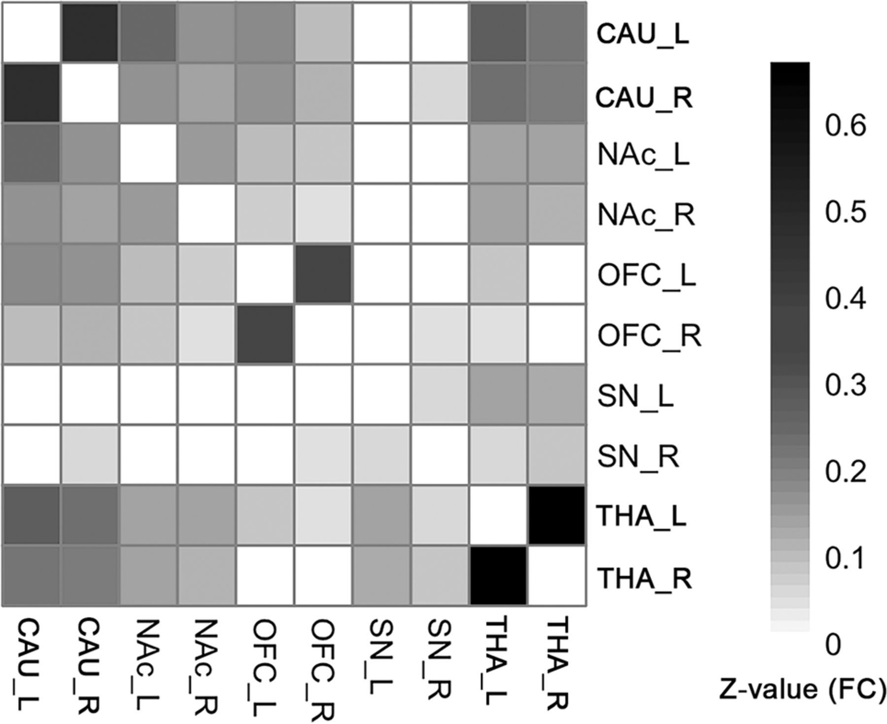
FCs existed between most of the ROI pairs. The FC pathways connecting bilateral CAU, bilateral NAc, bilateral OFC, bilateral THA, and bilateral SN were significant for all ROIs. The FC pathways between the left SN and bilateral CAU, bilateral NAc, bilateral OFC; the FC between the right SN and left CAU, bilateral NAc, left OFC; and between the right THA and bilateral OFC were not significant. All other FC pathways were significant except in the above-mentioned pathways (Fig 2, 1-sample t test, P < .05, FDR-corrected). The detailed statistical results of the 45 different FC pathways for the 10 ROIs can be found in the Online Supplemental Data.

The group-level FC matrix shows that the bilateral CAU, NAc, OFC, and THA ROIs are significantly connected to each other. The SN is significantly connected to the THA. Color represents the z-transformed FC strength between ROI pairs. White means statistically not significant (1-sample t test, P < .05, FDR-corrected). Note that if a connection was not significant, its representing FC was set to zero, to focus on the significant connections.
GC Analysis
The distribution of the GCI after 100,000 simulations is shown in Fig 3. The GCI density curve was skewed with a median value at 0.0163. The mu parameter in the Wilcoxon signed-rank test thus was set to 0.0163. If the GCI was significantly higher than mu, the corresponding GC connection was considered significant.

The GCI density curve. This curve comes from permutation-based technology to simulate the real-data GCI distribution with 100,000 times permutation. The distribution is a skewed curve, with 0.0163 as the median value, which is more appropriate than the mean value for the 1-sample test in this situation.
After multiple comparison correction, significant GC connections were as follows: a bidirectional connection between the left NAc and the right OFC and 8 significant unidirectional connections, respectively, from the right THA to the left CAU, from the left CAU to the right CAU, from the left CAU to the left OFC, from the left NAc to the left CAU, from the right OFC to the left CAU, from the left OFC to the right CAU, from the right NAc to the left OFC, and from the left OFC to the right OFC (Fig 4, 1-sample Wilcoxon signed-rank test, P < .05, FDR-corrected). The detailed data can be found in the Online Supplemental Data.

The group-wise directional network identified by GC. Arrows represent the direction of the pathways. The line thickness represents the relative strength of the GCI of that pathway. A bidirectional connection was identified between the right OFC and the left NAc (1-sample Wilcoxon signed-rank test, P < .05, FDR-corrected). L/R indicates left/right.
MCM Analysis
The significant MCM connection of the significant group-wise FC pathways were as follows: 3 bidirectional connections, respectively, between the bilateral THA, between the left CAU and the left NAc, and between the right CAU and the right NAc, and 7 unidirectional connections, respectively, from the left SN to the right THA, from the right OFC to the right CAU, from the left OFC to the bilateral CAU, from the right NAc to the bilateral CAU, and from the left CAU to the right CAU (Fig 5, 1-sample t test, P < .05, FDR-corrected). The detailed data can be found in the Online Supplemental Data.

The group-wise directional pathways identified by the MCM method. Arrows represent the direction of the pathways. The line thickness represents the relative strength of the MCM. There are more bidirectional interactions between the NAc and CAU, and the unidirectional pathway from the OFC to the CAU reveals the regulation in the frontostriatal DA pathway (1-sample t test, P < .05, FDR-corrected). L/R indicates left/right.
DISCUSSION
The GC and MCM methods were used to show differences in identifying directional connectivities of the DA brain reward system based on the Monash rsPET-MR data set. Our findings demonstrated that in the DA reward system, GC identified more cortico-nucleus bidirected connections and the MCM identified more directed connections among neighboring and symmetric regions. Each of the 2 methods has its own features, and researchers should carefully choose them before starting an analysis.
Both the GC and MCM identified modulation pathways in DA systems, but with different patterns. There are 3 major circuits in the DA reward system in the human brain: the basal ganglia (BG)–thalamocortical loop, the BG-thalamic loop, and the BG-habenulo-mesencephalic loop.18,31,35
GC revealed that the THA→CAU pathway belonged to the BG-thalamic loop and the OFC→NAc and CAU pathways belonged to the BG-thalamocortical loop. MCM revealed that the SN-to-THA pathway belonged to the BG-thalamic loop and the OFC→CAU pathways and the rich connections between CAU and NAc belonged to the BG-thalamocortical loop. These results are consistent with results from prior studies.18,31 The GC and MCM analytic approaches demonstrated the reliability of the 2 methods in revealing DA reward pathways. Neither GC or MCM analyses revealed the SN→limbic striatum pathway, implying that the sensitivities of the methods need to be improved. There were striatum→cortical pathways found by GC but not MCM, possibly caused by our omission of the existence of the THA mediation effect in our analysis.1 This result indicates that in the absence of a proper model, the GC analysis does not always identify specific pathways, while the MCM is not influenced.
GC analysis identified long-range connections (cortico-nucleus). The bidirected connections between the striatum and the OFC were identified by GC, consistent with the mesocortical pathway in the reward circuits.35 The MCM did well in identifying directed connections among neighboring brain areas (nucleus-nucleus) and among symmetric brain areas. These connections imply frequent communications between the dorsal and ventral striatum and the close communications between the bilateral subcortical brain areas in the resting-state brain.
The possible reason for the differences between GC and MCM may come from the different approaches of the 2 methods. The algorithm of the GC is based on a future temporal predictability from a knowledge of past activity.36 GC analytic results should be interpreted as predictions between time-series.2 If time-series X and Z have a high positive correlation, a high FC would result in a lower GC between X and Z because GC includes lags in its predictions between time-series and not correlations. For example, if X and Z are the same, there is no GC effect at all. In our results, the FC between the bilateral THA received the highest value, but there was no significant GC pathway between the bilateral THA. However, a high FC effect does not affect the ability of the MCM to identify this pathway because the algorithm of the MCM uses a voxelwise spatial pattern similarity between FDG and FC to generate the ROI-wise causality effect.3,9 The neighboring and symmetric brain regions often have higher FCs than long-distance brain regions. This inference is suggested by both observed phenomenologic and algorithmic differences.
Both the GC and MCM methods reported poor results for the subtentorial areas. The MCM identified the important projections from the SN to the THA and the interaction pathways between the bilateral THA. Our results showed that the SN and THA were isolated from the cortical areas and the striatum. However, it is known that the SN and THA have interactions with cortical areas and the striatum. The failure of the approaches to identify these interactions may be due to several factors: First, GC analysis does not work well in the midbrain/brainstem areas due to signal loss and image distortion of BOLD signals.37 GC analysis relies heavily on BOLD signal quality. High-resolution PET provided more benefit to MCM than GC. Second, the accuracy of the SN ROI template is limited because the SN is located in the midbrain and is more likely to have poor registration results than the cortex area using regular normalization procedures.37 Third, the correction method might be too stringent in 1-sample statistics compared with other studies that focused only on group differences in EC. For example, most of our GC studies calculated the between-group GC differences rather than within-group patterns, so we could test whether the group differences were significantly not equal to zero. When we focused on within-group patterns of GC, we had to choose a more stringent value to test. This strategy may have caused fewer identified results. The MCM, on the other hand, was less affected than GC when performing within-group analyses, resulting in a greater number of identified subtentorial areas than were identified by GC.
Considering the above methodological issues, MCM generally outperforms than GC in revealing reasonable directed connection in subcortical nucleus and cerebellum network. Thus, it is recommended that when the study aim at diseases involves mostly the subtentorial areas (e.g. cerebellum and subcortical nucleus), both FDG-PET and simultaneous BOLD data should be acquired and do MCM analysis.
This study has some limitations. First, the DA reward circuits involved ROIs that were arbitrarily selected and may have provided less comprehensive results. Second, the Monash rs-PET/MR data set acquired fMRI data using a TR = 2.45-second parameter, which may have limited the ability to identify DA pathways for GC. Third, the scan protocol of the Riedl et al9 study acquired 10-minute BOLD sequences immediately following the FDG injection, while the PET data used in our MCM analysis was collected 30 minutes after the FDG injection. In our study, the PET data represented the cumulated regional energy demands before the fMRI acquisition window, while the fMRI data reflected the neuronal dynamics during the acquisition phase. We assumed that the resting-state brain would have similar activities across sessions and that the FC would not change substantially, ensuring MCM stability. The stability of the MCM during the resting state in different sessions was not clear. Fourth, possible improvements to the original GC method,1,6,38 which may be more reliable, were not included in this study. Last, the present study comprised a small number of healthy participants (n = 27) only and was performed in a unique center; further studies could confirm the results with a larger sample size from multiple centers and validate the features in this study using patient data.
CONCLUSIONS
Our results showed that GC and MCM revealed different patterns in directional networks in the DA reward circuit. Our study demonstrated that both GC and the MCM could correctly identify some of the directed pathways among the DA reward circuits. GC identified long-range bidirected connections, and the MCM identified directed connections among neighboring and symmetric regions. Poor connections in subtentorial areas were identified by both methods, but MCM benefited from compensation of the high-resolution PET data. These results imply that future research on ECs requires an appropriate selection of methods according to the different objectives of the research.
Acknowledgment
The authors are grateful to S.D. Jamadar for sharing the OpenNeuro data set and to professor Riedl Valentin’s enthusiastic help with MCM methodology.
Footnotes
Lei Wang, Longxiao Wei and Yarong Wang contributed equally to this work.
This work was supported by grants from the National Natural Science Foundation of China (82071497 to Y. Wang).
Disclosure forms provided by the authors are available with the full text and PDF of this article at www.ajnr.org.
Indicates open access to non-subscribers at www.ajnr.org
References
- Received May 9, 2022.
- Accepted after revision October 1, 2022.
- © 2022 by American Journal of Neuroradiology


Jump to section
Related Articles
Cited By...
- No citing articles found.